Sample characteristics
Last updated 2022-01-04
Please cite these data with the following reference:
Condon, D. M., Coughlin, J., & Weston, S. J. (2022). Personality Trait Descriptors: 2,818 Trait Descriptive Adjectives characterized by familiarity, frequency of use, and prior use in psycholexical research. Journal of Open Psychology Data.
This page shows the demographic characteristics for the sample of participants who responded to the items. The sample contained participants from a wide range of ages, household incomes, and different geographies (by state) within the US. Note that residence in the US was a prerequisite for participation as the generalizability of the proportion of correct responses was intended to be limited to American English speakers only (i.e., not intended to extend to knowledge of American English terms among individuals residing outside of the US). Slightly more than half of the sample identified as female, roughly consistent with the US population. In terms of race/ethnicity (see figure below), the sample included a slightly higher proportion of participants identifying as White (73%) relative to the US population (64% of US adults according to the 2020 Census); the proportion of respondents identifying as Black or Hispanic was less than in the 2020 Census (9% vs 12% and 5% vs 16%, respectively). The majority had some college-level education (42%) or a high school degree/GED equivalent (40%).
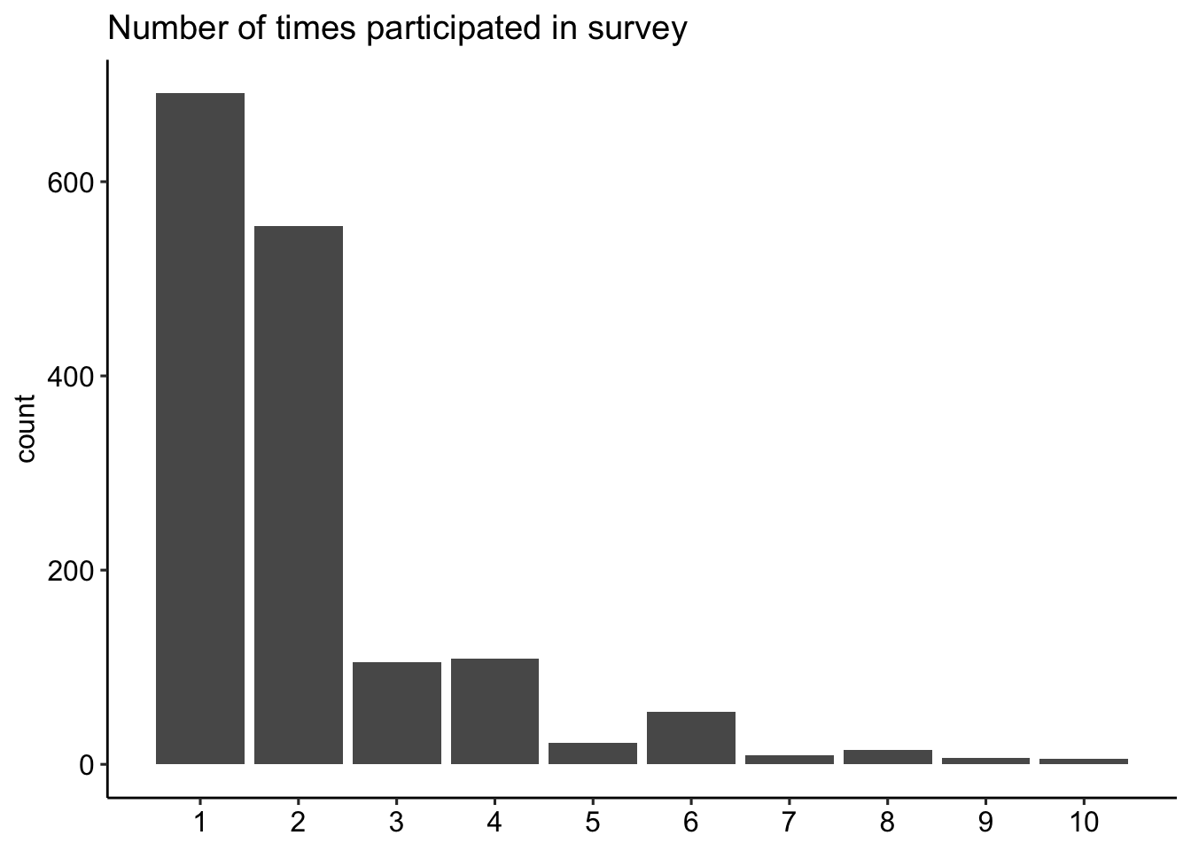
Note that most of the participants in the sample entered the survey through Prolific (90.7%); the remainder entered through Amazon’s Mechanical Turk platform. Participants were compensated at the US minimum wage rate (at the time of data collection) using the mean response time as an estimate of the time required. Participants were allowed to complete the survey multiple times, as each version of the survey contained only a small (random) subset of all possible terms. In other words, the possiblity of responding to the same item twice was low. The final figure on this page demonstrates that the majority of participants completed the survey only once (44%) or twice (35%). Across all 3,290 responses to the survey (1,572 unique respondents), participants answered an average of 73.4 items (median = 75).
The data can be downloaded here. NOTE that the csv version of these data will mis-read two adjectives when opened in MS Excel: “false” and “blasé”. These must be fixed manually prior to working with the data in Excel (but it appears to work as expected in R).
Please consult the reference listed above for more information about this project.
library(here)
library(ggpubr)
library(knitr)
library(maps)
library(conflicted)
library(tidyverse) # for data cleaning and manipulation
conflict_prefer("here", "here")
conflict_prefer("filter", "dplyr")
conflict_prefer("count", "dplyr")
conflict_prefer("mutate", "dplyr")


# Download the data manually from Dataverse using the doi link above
# data <- read.csv(here("data/TDA_data_scored.csv"))

# Or use the following lines to scrap the data file in directly
library(dataverse)
library(data.table)

Sys.setenv("DATAVERSE_SERVER" = "dataverse.harvard.edu")
writeBin(get_file("TDA_data_scored.tab", "doi:10.7910/DVN/5T80PF"), "TDA_data_scored.tab")
TDA_data_scored.tab <- fread("TDA_data_scored.tab", na.strings=getOption("<NA>","NA"))
data <- as.data.frame(TDA_data_scored.tab)
rm(TDA_data_scored.tab)

data = filter(data, included == "Yes")
data = data %>%
group_by(PID) %>%
dplyr::mutate(n = n())
data_part = data %>%
group_by(PID) %>%
filter(row_number() == 1) %>%
ungroup()Age
# Here we show code for analyzing the data by response instead of participant
# data %>%
#   ggplot(aes(x = age)) +
#   geom_histogram(binwidth = 1, color = "white") +
#   labs(title = "Age in years", x= NULL) +
#   theme_pubr()
data_part %>%
ggplot(aes(x = age)) +
geom_histogram(binwidth = 1, color = "white") +
labs(title = "Age in years", x= NULL) +
theme_pubr()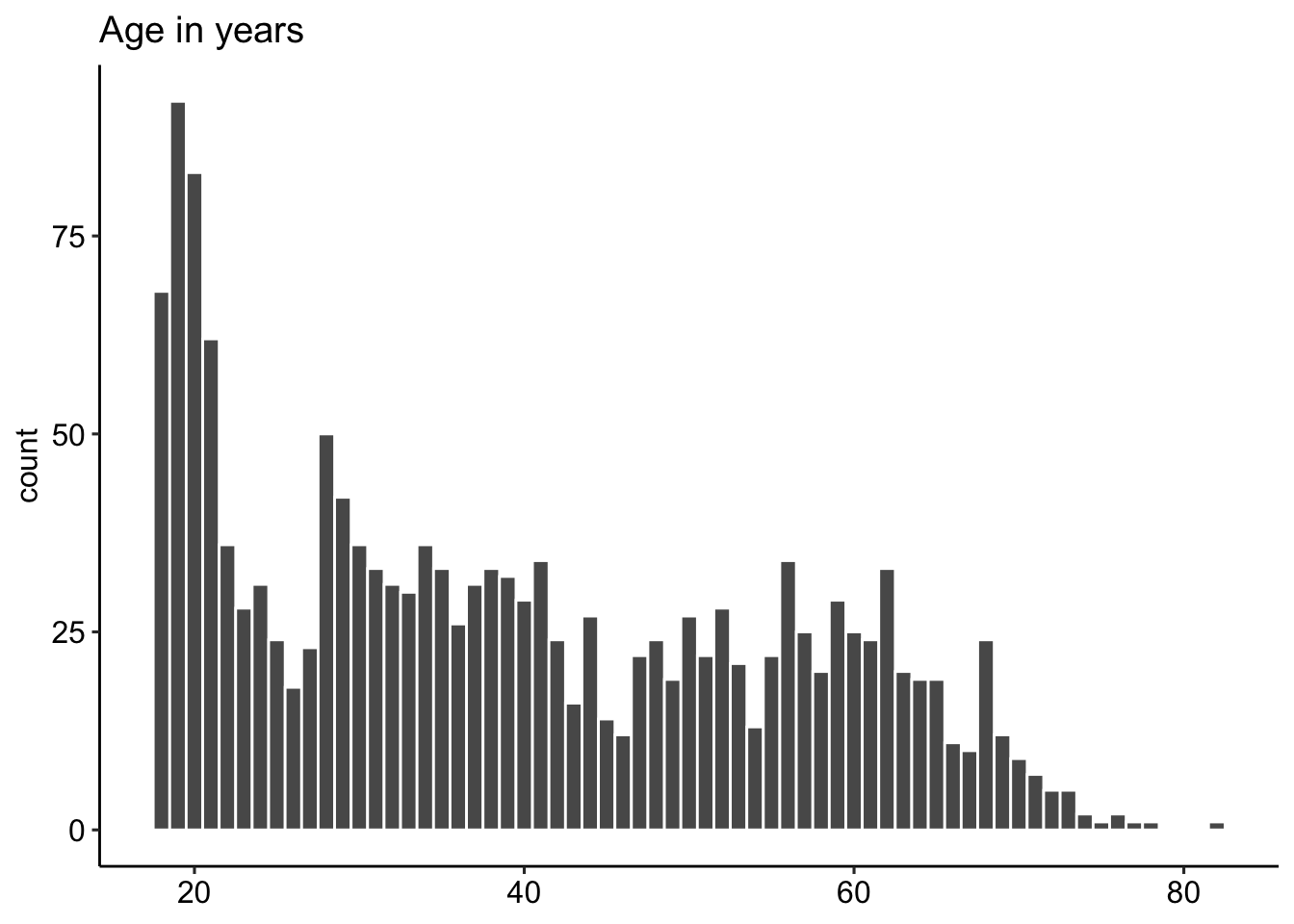
Sex
# Here we show code for analyzing the data by response instead of participant
# data %>%
#   group_by(sex) %>%
#   count() %>%
#   ungroup() %>%
#   dplyr::mutate(percent = 100*(n/sum(n)),
#          percent = round(percent),
#          percent = paste(percent, "%")) %>%
#   ggplot(aes(x = sex, y = n)) +
#   geom_bar(stat = "identity") +
#   geom_text(aes(label = percent), vjust = 0) +
#   labs(title = "What was your biological sex at birth", x= NULL) +
#   theme_pubr()
data_part %>%
group_by(sex) %>%
count() %>%
ungroup() %>%
dplyr::mutate(percent = 100*(n/sum(n)),
percent = round(percent),
percent = paste(percent, "%")) %>%
ggplot(aes(x = sex, y = n)) +
geom_bar(stat = "identity") +
geom_text(aes(label = percent), vjust = 0) +
labs(title = "What was your biological sex at birth", x= NULL) +
theme_pubr()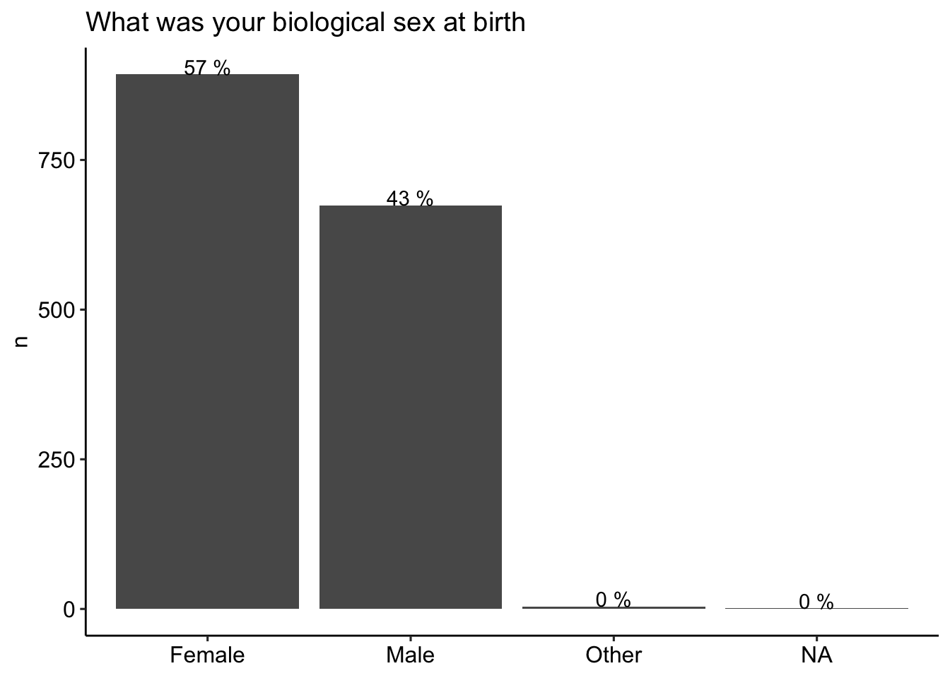
Education
# Here we show code for analyzing the data by response instead of participant
# data %>%
#   dplyr::mutate(edu = factor(edu, levels = c(
#       "Less than 12 years",
#       "High school grad/GED",
#       "Currently in college/university",
#       "Some college/university, but did not graduate",
#       "Associate degree (2 yr)",
#       "College/university degree (4 yr)",
#       "Currently in grad/professional school",
#       "Grad/professional degree"
#   ))) %>%
#   group_by(edu) %>%
#   count() %>%
#   ungroup() %>%
#   dplyr::mutate(percent = 100*(n/sum(n)),
#          percent = round(percent),
#          percent = paste(percent, "%")) %>%
#   ggplot(aes(x = edu, y = n)) +
#   geom_bar(stat = "identity") +
#   geom_text(aes(label = percent), vjust = 0) +
#   labs(title = "Level of education", x= NULL) +
#   theme_pubr() +
#   theme(axis.text.x = element_text(angle = 65, vjust =1, hjust = 1))
data_part %>%
dplyr::mutate(edu = factor(edu, levels = c(
"Less than 12 years",
"High school grad/GED",
"Currently in college/university",
"Some college/university, but did not graduate",
"Associate degree (2 yr)",
"College/university degree (4 yr)",
"Currently in grad/professional school",
"Grad/professional degree"
))) %>%
group_by(edu) %>%
count() %>%
ungroup() %>%
dplyr::mutate(percent = 100*(n/sum(n)),
percent = round(percent),
percent = paste(percent, "%")) %>%
ggplot(aes(x = edu, y = n)) +
geom_bar(stat = "identity") +
geom_text(aes(label = percent), vjust = 0) +
labs(title = "Level of education", x= NULL) +
theme_pubr() +
theme(axis.text.x = element_text(angle = 65, vjust =1, hjust = 1))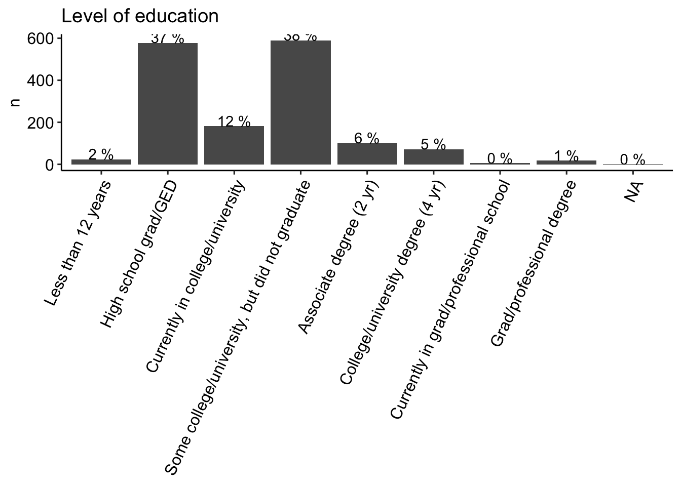
Ethnicity
# Here we show code for analyzing the data by response instead of participant
# data %>%
#   dplyr::mutate(ethnic = factor(ethnic, levels = c(
#      "American Indian/Alaskan Native",
#      "Asian",
#      "Black",
#      "Hispanic",
#      "White",
#      "Mixed (two or more)",
#      "Other"
#   ))) %>%
#   group_by(ethnic) %>%
#   count() %>%
#   ungroup() %>%
#   dplyr::mutate(percent = 100*(n/sum(n)),
#          percent = round(percent),
#          percent = paste(percent, "%")) %>%
#   ggplot(aes(x = ethnic, y = n)) +
#   geom_bar(stat = "identity") +
#   geom_text(aes(label = percent), vjust = 0) +
#   labs(title = "Racial/ethnic identity", x= NULL) +
#   theme_pubr() +
#   theme(axis.text.x = element_text(angle = 65, vjust =1, hjust = 1))
data_part %>%
dplyr::mutate(ethnic = factor(ethnic, levels = c(
"American Indian/Alaskan Native",
"Asian",
"Black",
"Hispanic",
"White",
"Mixed (two or more)",
"Other"
))) %>%
group_by(ethnic) %>%
count() %>%
ungroup() %>%
dplyr::mutate(percent = 100*(n/sum(n)),
percent = round(percent),
percent = paste(percent, "%")) %>%
ggplot(aes(x = ethnic, y = n)) +
geom_bar(stat = "identity") +
geom_text(aes(label = percent), vjust = 0) +
labs(title = "Racial/ethnic identity", x= NULL) +
theme_pubr() +
theme(axis.text.x = element_text(angle = 65, vjust =1, hjust = 1))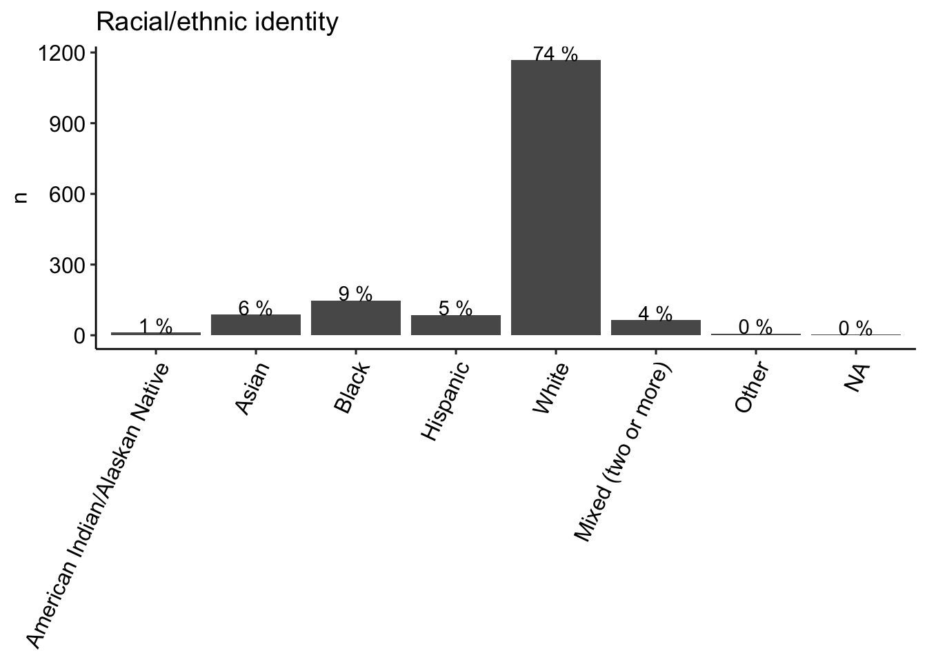
Household income
# Here we show code for analyzing the data by response instead of participant
# data %>%
#   dplyr::mutate(hhinc = factor(hhinc, levels = c(
#       "< 20K",
#       "20K-40K",
#       "40K-60K",
#       "60K-80K",
#       "80K-100K",
#       "100K-120K",
#       "120K-150K",
#       "150K-200K",
#       "200K-250K",
#        "250K-350K",
#        "350K-500K",
#        "> 500K"
#   ))) %>%
#   group_by(hhinc) %>%
#   count() %>%
#   ungroup() %>%
#   dplyr::mutate(percent = 100*(n/sum(n)),
#          percent = round(percent),
#          percent = paste(percent, "%")) %>%
#   ggplot(aes(x = hhinc, y = n)) +
#   geom_bar(stat = "identity") +
#   geom_text(aes(label = percent), vjust = 0) +
#   labs(title = "Household Income", x= NULL) +
#   theme_pubr() +
#   theme(axis.text.x = element_text(angle = 65, vjust =1, hjust = 1))
data_part %>%
dplyr::mutate(hhinc = factor(hhinc, levels = c(
"< 20K",
"20K-40K",
"40K-60K",
"60K-80K",
"80K-100K",
"100K-120K",
"120K-150K",
"150K-200K",
"200K-250K",
"250K-350K",
"350K-500K",
"> 500K"
))) %>%
group_by(hhinc) %>%
count() %>%
ungroup() %>%
dplyr::mutate(percent = 100*(n/sum(n)),
percent = round(percent),
percent = paste(percent, "%")) %>%
ggplot(aes(x = hhinc, y = n)) +
geom_bar(stat = "identity") +
geom_text(aes(label = percent), vjust = 0) +
labs(title = "Household Income", x= NULL) +
theme_pubr() +
theme(axis.text.x = element_text(angle = 65, vjust =1, hjust = 1))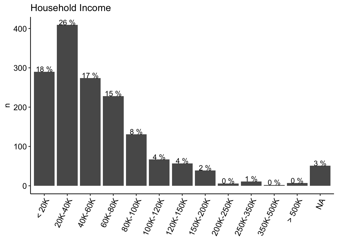
State of residence
N by state
data_part %>%
  filter(!is.na(state)) %>%
  group_by(state) %>%
  count() %>%
  ggplot(aes(x = reorder(state, n), y = n)) +
  geom_bar(stat = "identity") +
  labs(x = NULL, y = "Count") +
  coord_flip() +
theme_pubr() 
Map
MainStates <- map_data("state")

data_part %>%
  with_groups(state, count) %>%
  dplyr::mutate(region = tolower(state)) %>%
  inner_join(MainStates) %>%
  ggplot() +
  geom_polygon(aes(x=long, y=lat, group=group, fill = n),
                color="black") +
  scale_x_continuous(breaks = NULL) +
  scale_y_continuous(breaks = NULL) +
  scale_fill_gradient(low = "white", high = "darkblue") +
  labs(x = NULL, y = NULL) +
  theme_pubr()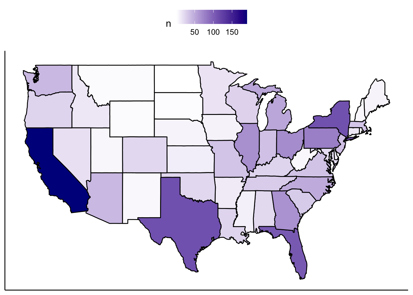
Participant response rates
data %>%
  group_by(PID) %>%
  count() %>%
  ggplot(aes(x = n)) +
  geom_bar(stat = "count") +
  scale_x_continuous(breaks = 1:13) +
  labs(title = "Number of times participated in survey",
       x = NULL) +
  theme_pubr()