Data cleaning
Last updated 2023-08-11
The current section documents the data cleaning process.
0.1 Workspace
library(here) # for working with files
library(tidyverse) # for cleaning
library(janitor) # for variable names
library(stringi) # for generating random strings
library(glmmTMB) # for multilevel modeling
library(broom) # for presenting results
library(sjPlot) # for figures
library(ggpubr) # for prettier plots
library(kableExtra) # for nicer tables
library(stringdist) # for scoring memory task
library(papaja) # for pretty numbers
library(psych) # for correlation tests
library(broom.mixed) # for tidying multilevel models
0.2 Change participant ID values
Before we begin, we create new versions of each data_t1 file that can be shared for purposes of reproducibility. These data_t1 files do not include variables that contain potentially identifying meta-data_t1 (e.g., IP address, latitude and longitude). Importantly, we also replace all Prolific ID values with new, random strings, to prevent the possibility that these participants are later identified. We also fix an error that can be introduced through Qualtrics, specifically that all or parts of the text string “Value will be set from panel or URL” is sometimes entered into the text box for ID. Prolific ID values are always 24 characters long and start with a number – we search for strings that meet this criteria.
(We note that the code chunks in this subsection are turned off in the RMarkdown file – eval = F – as readers will not be able to run these chunks.)
# function to load raw file, clean the names, and remove meta-data_t1
# creating a function ensures the same procedure is applied to all
# orginal datasets

load_data = function(path){

  full_path = here(path)
  data_obj  = read_rds(path)

  data_obj = clean_names(data_obj)

  data_obj = data_obj %>%
    select(-end_date,
           -ip_address,
           -progress,
           -finished,
           -recorded_date,
           -status,
           -response_id,
           -external_reference,
           -distribution_channel,
           -user_language,
           -starts_with("recipient"),
           -starts_with("location"),
           -starts_with("meta_info"),
           -prolific_pid)

  data_obj = data_obj %>%
    mutate(proid = str_extract(proid, "\\d([[:alnum:]]{23})"))

  return(data_obj)
}

data_t1 <- load_data("data/data_t1.rds")
data_2A <- load_data("data/data_2A.rds")
data_2B <- load_data("data/data_2B.rds")
data_2C <- load_data("data/data_2C.rds")
data_2D <- load_data("data/data_2D.rds")
0.3 Manually update entries
Several participants notified us of mistaken answers after completing the survey. We fix those entries here.
data_t1$sex[data_t1$proid == "63b7d7a4ab0b515649d4f4de"] = "Female"
data_t1$devicetype[data_t1$proid == "60da4f9aa1ced7efeecca18a"] = "Tablet (for example, iPad, Galaxy Tablet, Amazon Fire, etc.)"
data_t1$inaccurate_responses[data_t1$proid == "60da4f9aa1ced7efeecca18a"] = "No"
0.4 Deidentify data – only run after data collection is complete
We identify all unique participant IDs. For each, we generate a new string, Then we replace the original ID values with the new strings.
original_id <- unique(c(data_t1$proid,
                       data_2A$proid,
                       data_2B$proid,
                       data_2C$proid,
                       data_2D$proid))

#remove missing values -- represent bots or tests
original_id = original_id[!is.na(original_id)]

#generate new ids (randoms tring of letters and numbers)
set.seed(202108)
new_id <- stri_rand_strings(n = length(original_id), length = 24)

#replace old string with new string
for(i in 1:length(original_id)){
  data_t1$proid[data_t1$proid == original_id[i]] <- new_id[i]
  data_2A$proid[data_2A$proid == original_id[i]] <- new_id[i]
  data_2B$proid[data_2B$proid == original_id[i]] <- new_id[i]
  data_2C$proid[data_2C$proid == original_id[i]] <- new_id[i]
  data_2D$proid[data_2D$proid == original_id[i]] <- new_id[i]
}
We end by saving each data_t1 frame as new .csv files, to be uploaded to OSF and shared for reproduction.
write_csv(data_t1, file = here("deidentified data/data_time1.csv"))
write_csv(data_2A, file = here("deidentified data/data_time2_A.csv"))
write_csv(data_2B, file = here("deidentified data/data_time2_B.csv"))
write_csv(data_2C, file = here("deidentified data/data_time2_C.csv"))
write_csv(data_2D, file = here("deidentified data/data_time2_D.csv"))
data_t1 <- read_csv(here("deidentified data/data_time1.csv"))
data_2A <- read_csv(here("deidentified data/data_time2_A.csv"))
data_2B <- read_csv(here("deidentified data/data_time2_B.csv"))
data_2C <- read_csv(here("deidentified data/data_time2_C.csv"))
data_2D <- read_csv(here("deidentified data/data_time2_D.csv"))0.5 Time 1
We rename several columns, in order to facilitate the use of regular expressions later. Specifically, we remove the underscores (_) in the columns pertaining to broad-mindedness and self-disciplined.
names(data_t1) = str_replace(names(data_t1), "broad_mind", "broadmind")
names(data_t1) = str_replace(names(data_t1), "self_disciplind", "selfdisciplined")
We can also remove the meta-data (timing, etc) around two attention check adjectives, “human” and “asleep”.
data_t1 = data_t1 %>%
  select(-starts_with("t_human"),
         -starts_with("t_asleep"))
0.5.1 Recode personality item responses to numeric
We recode the responses to personality items, which we downloaded as text strings. We chose to use text strings as opposed to numbers to avoid any possibility that the Qualtrics-set coding was incorrect. We start this process by identifying the personality items (p_items) using regular expressions. All personality items take a format like outgoing_a or helpful_b_2; that is, they start with the adjective, followed by a letter indicating with which condition or item format the adjective was presented, and sometimes they are followed by a 2, indicating it was the second time the participant saw the adjective. We can represent this pattern using regular expressions.
p_items = str_extract(names(data_t1), "^[[:alpha:]]*_[abcd](_2)?$")
p_items = p_items[!is.na(p_items)]

personality_items = select(data_t1, proid, all_of(p_items))
Next, we write a simple function to recode values. We find the case_when function to be the most clear method of communicating the recoding process when moving from string to numeric.
recode_p = function(x){
  y = case_when(
    x == "Very inaccurate" ~ 1,
    x == "Moderately inaccurate" ~ 2,
    x == "Slightly inaccurate" ~ 3,
    x == "Slightly accurate" ~ 4,
    x == "Moderately accurate" ~ 5,
    x == "Very accurate" ~ 6,
    TRUE ~ NA_real_)
  return(y)
}
Finally, we apply this function to all personality items.
personality_items = personality_items %>%
  # apply to all variables except proid
  mutate(across(!c(proid), recode_p))
Now we merge the recoded values back into the data_t1.
# remove personality items from data file
data_t1 = select(data_t1, -all_of(p_items))
# merge in recoded personality items
data_t1 = full_join(data_t1, personality_items)
0.5.2 Drop bots and inattentive participants
0.5.2.1 Based on ID
Recall that when preparing the data files for sharing, we replaced all Prolific IDs with random strings. A consequence of this cleaning is that any ID entered that did not have a string meeting the Prolific ID format requirements (24 character, starting with a number) was replaced with NA. To remove these bots, we can simply filter out missing ID values.
We removed 0 participants without valid Prolific IDs. (This likely occurred based on sharing of the survey link among Prolific users.)
0.5.2.2 Based on language
data_t1 = data_t1 %>%
  filter(english %in% c("Well", "Very well (fluent/native)"))
We removed 1 participants that do not speak english well or very well.
0.5.2.3 Based on inattentive responding
We expect to exclude any participant who has an average response of 4 (“slightly agree”) or greater to the attention check items. Two items from the Inattentive and Deviant Responding Inventory for Adjectives (IDRIA) scale (Kay & Saucier, in prep) have been included here, in part to help evaluate the extent of inattentive responding but also to consider the effect of item wording on these items. The two items used here (i.e., “Asleep”, “Human”) were chosen to be as inconspicuous as possible, so as to not to inflate item response duration. The frequency item (i.e., “human”) will be reverse-scored, so that higher scores on both the infrequency and frequency items reflect greater inattentive responding. Figure 1 shows the distribution of average responses to attention check items.
in_average = data_t1 %>%
  # reverse score human
  mutate(across(matches("^human"),  ~(.x*-1)+7)) %>%
  # select id and attention check items
  select(proid, matches("^human"), matches("^asleep")) %>%
  gather(item, response, -proid) %>%
  filter(!is.na(response)) %>%
  group_by(proid) %>%
  summarise(avg = mean(response)) %>%
  mutate(
    remove = case_when(
      avg >= 4 ~ "Remove",
      TRUE ~ "Keep"))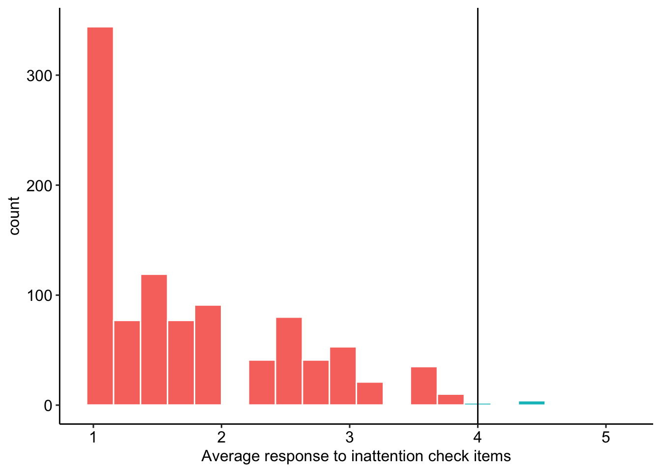
Figure 1: Average response to inattention check items
We remove 8 participants whose responses suggest inattention.
data_t1 = data_t1 %>%
  full_join(select(in_average, proid, remove)) %>%
  filter(remove != "Remove") %>%
  select(-remove)
0.5.2.4 Based on patterns
We remove any participant who provides the same response to over half of the items (21 or more items) from a given block in a row.
To proceed, first we create a data frame containing just the responses to personality items in the first block.
# first, identify unique adjectives, in order
adjectives = p_items %>%
  str_remove_all("_.") %>%
  unique()

# extract block 1 questions using regular expressions
# these follow the personality item format described above, but never end with 2
block1 = data_t1 %>%
  select(proid, matches("^[[:alpha:]]+_[abcd]$"))
Next, we rename the variables. Instead of variable names identifying the specific adjective (e.g., outgoing_a), we need variable names which indicate the order in which the adjective was seen by the participant (e.g., trait01_a). This will help us determine patterns by item order, rather than adjective content. Participants all saw adjectives in the same order (i.e., all participants, regardless of condition, saw outgoing first).
#rename variables
n = 0
for(i in adjectives){ # for each adjective
  n = n+1 # identify its location in the presentation
  names(block1) = str_replace(names(block1), #in variable names
                              # replace the adjective string
                              i,
                              # with the word trait followed by its place
                              paste0("trait", str_pad(n, 2, pad = "0")))
}
We use gather and spread to quickly combine columns measuring the same trait. That is, instead of having columns trait01_a, trait01_b, trait01_c, and trait01_d, we now have a single column called trait01.
block1 = block1 %>%
  gather(item, response, -proid) %>%
  filter(!is.na(response)) %>%
  separate(item, into = c("item", "format")) %>%
  select(-format) %>%
  spread(item, response)
To count the number of runs, we loop through participants and, within participant, loop through columns. Within participant, we create an object called run. If a response to a personality item is the same as the participant’s response to the previous item, we increase the value of run by 1. If this new value is the largest run value for that participant, it becomes the value of an object called maxrun. If the participant gives a new response, run is reset to 0. We record the maxrun value for each partipant in a variable called block1_runs.
block1_runs = numeric(length = nrow(block1))


for(i in 1:nrow(block1)){
  run = 0
  maxrun = 0
  for(j in 3:ncol(block1)){
    if(block1[i,j] == block1[i, j-1]){
      run = run+1
      if(run > maxrun) maxrun = run
      } else{ run = 0}
  }
  block1_runs[i] = maxrun
}

#add to data_t1 frame
block1$block1_runs = block1_runs
Here we repeat the process described above with Block 2 data.
# extract block 2 questions
block2 = data_t1 %>%
  select(proid, matches("^[[:alpha:]]+_[abcd]_2$"))

#rename variables
n = 0
for(i in adjectives){
  n = n+1
  names(block2) = str_replace(names(block2), i, paste0("trait", str_pad(n, 2, pad = "0")))
}

block2 = block2 %>%
  gather(item, response, -proid) %>%
  filter(!is.na(response)) %>%
  mutate(item = str_remove(item, "_2")) %>%
  separate(item, into = c("item", "format")) %>%
  select(-format) %>%
  spread(item, response)

block2_runs = numeric(length = nrow(block2))

#identify max run for each participant
for(i in 1:nrow(block2)){
  run = 0
  maxrun = 0
  for(j in 3:ncol(block2)){
    if(block2[i,j] == block2[i, j-1]){
      run = run+1
      if(run > maxrun) maxrun = run
      } else{ run = 0}
  }
  block2_runs[i] = maxrun
}

#add to data_t1 frame
block2$block2_runs = block2_runs
We combine the variables holding the maximum runs into a single data frame. We will remove participants if their maximum run in either block was greater than or equal to 21. See Figure 2 for a visualization of the spread and associations between run lengths across participants.
#combine results
runs_data = block1 %>%
  select(proid, block1_runs) %>%
  full_join(select(block2, proid, block2_runs)) %>%
  mutate(
    remove = case_when(
      block1_runs >= 21 ~ "Remove",
      block2_runs >= 21 ~ "Remove",
      TRUE ~ "Keep"
    ))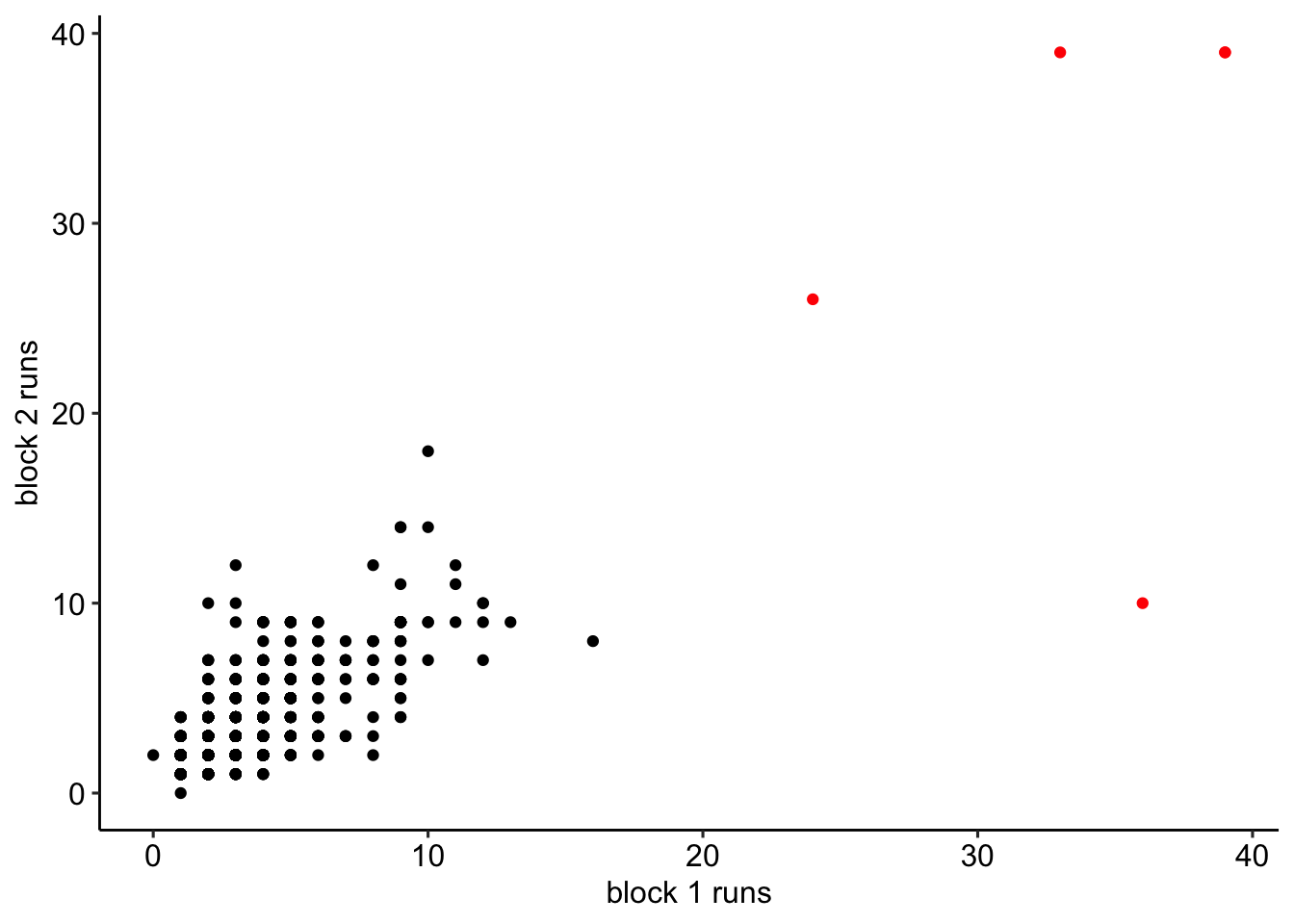
Figure 2: Maximum number of same consecutive responses in personality blocks.
There were 5 participants who provided the same answer 21 or more times in a row. These participants were removed from the analyses.
data_t1 = data_t1 %>%
  full_join(select(runs_data, proid, remove)) %>%
  filter(remove != "Remove") %>%
  select(-remove)

rm(runs_data)
0.5.2.5 Based on average time to respond to personality items
First, select just the timing of the personality items. We do this by searching for specific strings: “t_[someword][a or b or c or d](maybe 2_)_page_submit.”
timing_data = data_t1 %>%
  select(proid, matches("t_[[:alpha:]]*_[abcd](_2)?_page_submit"))
Next we gather into long form and remove missing timing values
timing_data = timing_data %>%
  gather(variable, timing, -proid) %>%
  filter(!is.na(timing))
To check, each participant should have the same number of responses: 76.
timing_data %>%
  group_by(proid) %>%
  count() %>%
  ungroup() %>%
  summarise(min(n), max(n))
## # A tibble: 1 × 2
## `min(n)` `max(n)`
## <int> <int>
## 1 76 76Excellent! Now we calculate the average response time per item for each participant. We mark a participant for removal if their average time is less than 1 second or greater than 30. See Figure 3 for a distribution of average response time.
timing_data = timing_data %>%
  group_by(proid) %>%
  summarise(m_time = mean(timing)) %>%
  mutate(remove = case_when(
    m_time < 1 ~ "Remove",
    m_time > 30 ~ "Remove",
    TRUE ~ "Keep"
  ))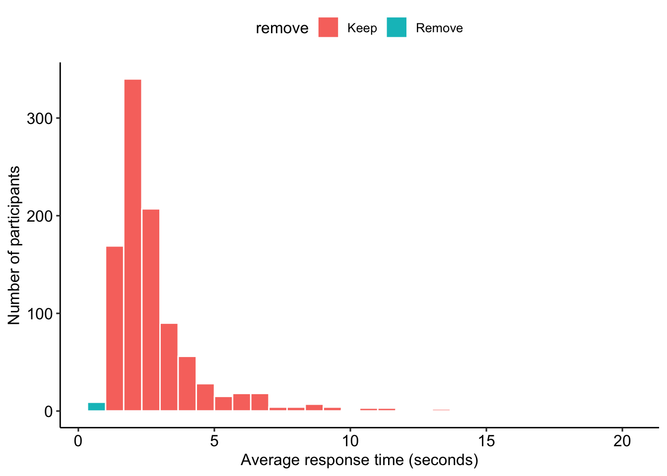
Figure 3: Distribution of average time to respond to personality items.
data_t1 = inner_join(data_t1, filter(timing_data, remove == "Keep")) %>%
  select(-remove)
Based on timing, we removed 9 participants.
We create a variable which indicates the Block 1 condition of each participant. This is used in two places: first, in recruiting participants at Time 2 (participants are given the same format at Time 2 as they received in Block 1), and second, in selecting the corret items during the test-retest analyses.
data_t1 = data_t1 %>%
  mutate(condition = case_when(
    !is.na(outgoing_a) ~ "A",
    !is.na(outgoing_b) ~ "B",
    !is.na(outgoing_c) ~ "C",
    !is.na(outgoing_d) ~ "D",
  ))
At this point, we’ll extract the Prolific ID numbers. These participants will be eligible to take the survey at Time 2.
data_t1 %>%
  select(proid, condition) %>%
  write_csv(file = here("data/elligible_proid.csv"))
0.6 Time 2
data_2 = data_2A %>%
  full_join(data_2B) %>%
  full_join(data_2C) %>%
  full_join(data_2D)
Rename the following columns.
data_2 = data_2 %>%
  rename(start_date2 = start_date,
         duration_in_seconds2 = duration_in_seconds)
We rename several columns, in order to facilitate the use of regular expressions later. Specifically, we remove the underscores (_) in the columns pertaining to broad-mindedness and self-disciplined.
names(data_2) = str_replace(names(data_2), "broad_mind", "broadmind")
names(data_2) = str_replace(names(data_2), "self_disciplind", "selfdisciplined")
We can also remove the meta-data (timing, etc) around two attention check adjectives, “human” and “asleep”.
data_2 = data_2 %>%
  select(-starts_with("t_human"),
         -starts_with("t_asleep"))
0.6.1 Recode personality item responses to numeric
We recode the responses to personality items, which we downloaded as text strings. Here, all items end with _3 and sometimes with i.
p_items_2 = str_extract(names(data_2), "^[[:alpha:]]*_[abcd]_3(i)?$")
p_items_2 = p_items_2[!is.na(p_items_2)]

personality_items_2 = select(data_2, proid, all_of(p_items_2))
We apply the recoding function to all personality items.
personality_items_2 = personality_items_2 %>%
  mutate(
    across(!c(proid), recode_p))
Now we merge this back into the data_2.
data_2 = select(data_2, -all_of(p_items_2))
data_2 = full_join(data_2, personality_items_2)
0.6.2 Drop bots and inattentive participants
This code recreates the steps outlined in detail above for Time 1. Please refer to the descriptions above for justification and explaination of the code presented here.
0.6.2.1 Based on ID
We also check that the ID in time 2 matches an ID in time 1.
data_2 = data_2 %>%
  filter(proid %in% data_t1$proid)
We removed 2 participants without valid Prolific IDs.
0.6.2.2 Based on inattentive responding
Participants who respond positively to the adjective asleep or negatively to the word human are assumed to be inattentive. We filter out participants whose average response to these two items is greater than or equal to 4 (see Figure 4 for the distribution).
in_average = data_2 %>%
  # reverse score human
  mutate(across(matches("^human"),  ~(.x*-1)+7)) %>%
  # select id and attention check items
  select(proid, matches("^human"), matches("^asleep")) %>%
  gather(item, response, -proid) %>%
  filter(!is.na(response)) %>%
  group_by(proid) %>%
  summarise(avg = mean(response)) %>%
  mutate(
    remove = case_when(
      avg >= 4 ~ "Remove",
      TRUE ~ "Keep"))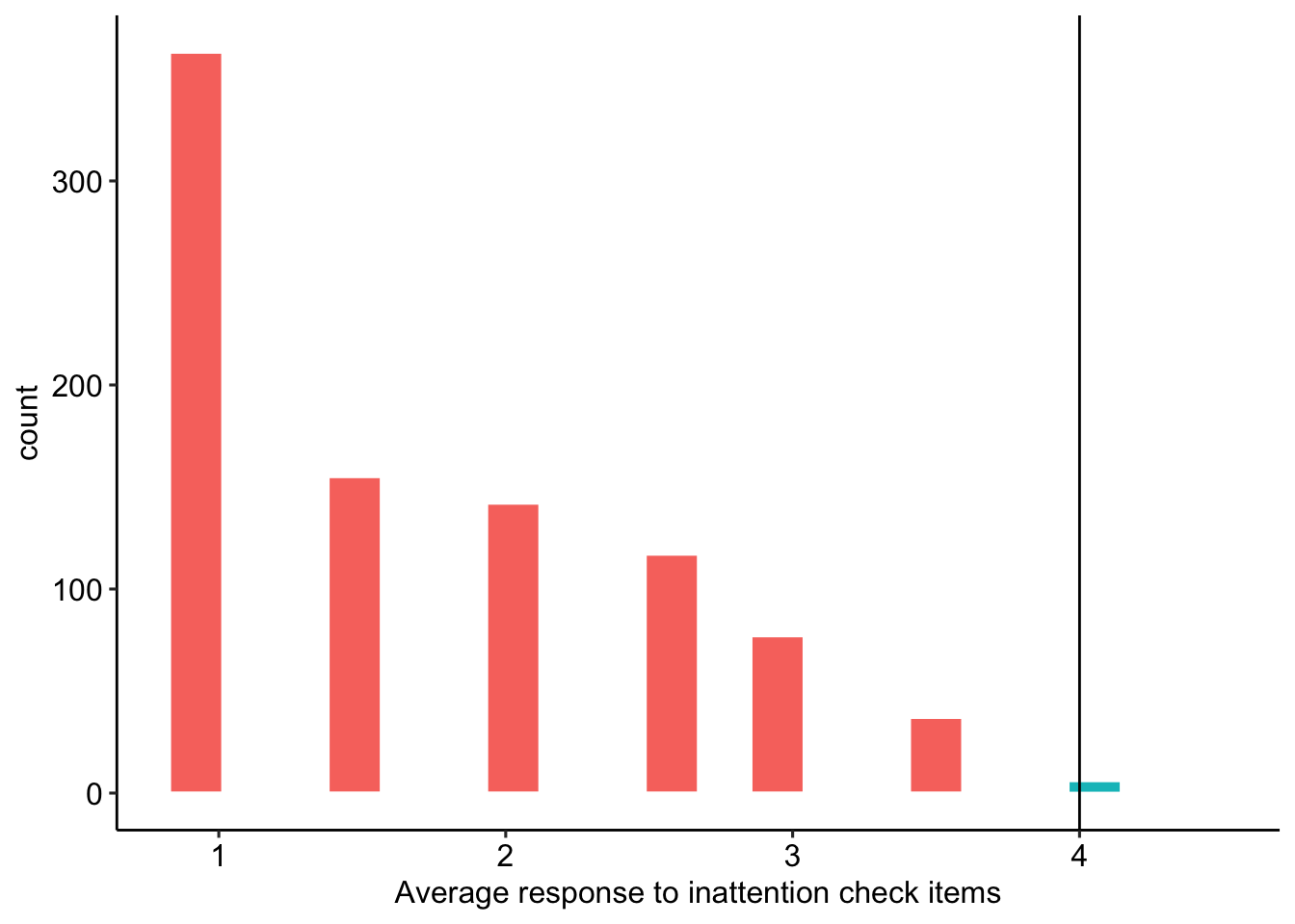
Figure 4: Average response to inattention check items
We remove 7 participants whose responses suggest inattention.
data_2 = data_2 %>%
  full_join(select(in_average, proid, remove)) %>%
  filter(remove != "Remove") %>%
  select(-remove)
0.6.2.3 Based on patterns
We remove any participant who provides the same response to over half of the items (21 or more items) from a given block in a row. The distribution of runs in Time 2 is depicted in Figure 5.
# first, identify unique adjectives, in order
adjectives = p_items_2 %>%
  str_remove_all("_.") %>%
  unique()

# extract block 3 questions
block3 = data_2 %>%
  select(proid, all_of(p_items_2))

#rename variables
n = 0
for(i in adjectives){
  n = n+1
  names(block3) = str_replace(names(block3), i, paste0("trait", str_pad(n, 2, pad = "0")))
}


block3 = block3 %>%
  gather(item, response, -proid) %>%
  filter(!is.na(response)) %>%
  mutate(item = str_remove(item, "_3(i)?$")) %>%
  separate(item, into = c("item", "format")) %>%
  select(-format) %>%
  spread(item, response)

block3_runs = numeric(length = nrow(block3))

for(i in 1:nrow(block3)){
  run = 0
  maxrun = 0
  for(j in 3:ncol(block3)){
    if(block3[i,j] == block3[i, j-1]){
      run = run+1
      if(run > maxrun) maxrun = run
      } else{ run = 0}
  }
  block3_runs[i] = maxrun
}

#add to data_2 frame
block3$block3_runs = block3_runs
#combine results
runs_data_2 = block3 %>%
select(proid, block3_runs) %>%
mutate(
remove = case_when(
block3_runs >= 21 ~ "Remove",
TRUE ~ "Keep"
))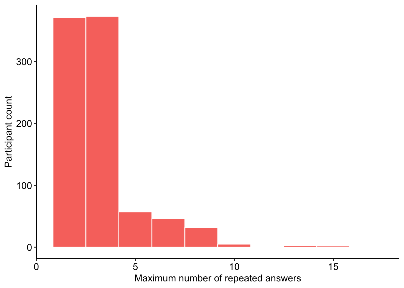
Figure 5: Maximum number of same consecutive responses in personality block 3.
There were 0 participants who provided the same answer 21 or more times in a row. These participants were removed from the analyses.
data_2 = data_2 %>%
  full_join(select(runs_data_2, proid, remove)) %>%
  filter(remove != "Remove") %>%
  select(-remove)

rm(runs_data_2)
0.6.2.4 Based on average time to respond to personality items
Participants who take too little (< 1 second) or too long (greater than 30 seconds) on average to answer each personality item are excluded. See Figure 6 for the distribution of average response time per item.
timing_data_2 = data_2 %>%
  select(proid, matches("t_[[:alpha:]]*_[abcd]_3(i)?_page_submit"))

timing_data_2 = timing_data_2 %>%
  gather(variable, timing, -proid) %>%
  filter(!is.na(timing))
To check, each participant should have the same number of responses: 33.
timing_data_2 %>%
  group_by(proid) %>%
  count() %>%
  ungroup() %>%
  summarise(min(n), max(n))
## # A tibble: 1 × 2
## `min(n)` `max(n)`
## <int> <int>
## 1 37 38timing_data_2 = timing_data_2 %>%
group_by(proid) %>%
summarise(m_time = mean(timing)) %>%
mutate(remove = case_when(
m_time < 1 ~ "Remove",
m_time > 30 ~ "Remove",
TRUE ~ "Keep"
))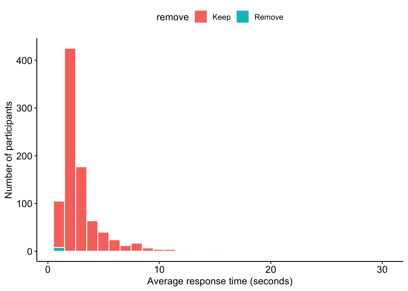
Figure 6: Distribution of average time to respond to personality items in Block 3.
data_2 = inner_join(data_2, filter(timing_data_2, remove == "Keep")) %>%
  select(-remove)
Based on timing, we removed 8 participants.
0.6.3 Merge all datasets together
We merge the Time 1 and Time 2 datasets together here.
data_2 = data_2 %>%
  select(proid, start_date2, duration_in_seconds2, very_delayed_recall, contains("_3")) %>%
  mutate(time2 = "yes") #indicates participant in time 2

data = data_t1 %>% full_join(data_2)
0.7 All data
0.7.1 Reverse score personality items
The following items are (typically) negatively correlated with the others: reckless, moody, worrying, nervous, careless, impulsive. We reverse-score them to ease interpretation of associations and means in the later sections. In short, all traits will be scored such that larger numbers are indicative of the more socially desirable end of the spectrum.
data = data %>%
  mutate(
    across(matches("^reckless"),       ~(.x*-1)+7),
    across(matches("^moody"),          ~(.x*-1)+7),
    across(matches("^worrying"),       ~(.x*-1)+7),
    across(matches("^nervous"),        ~(.x*-1)+7),
    across(matches("^careless"),       ~(.x*-1)+7),
    across(matches("^impulsive"),      ~(.x*-1)+7),
    across(matches("^quiet"),          ~(.x*-1)+7),
    across(matches("^unsympathetic"),  ~(.x*-1)+7),
    across(matches("^uncreative"),     ~(.x*-1)+7),
    across(matches("^shy"),            ~(.x*-1)+7),
    across(matches("^cold"),           ~(.x*-1)+7),
    across(matches("^unintellectual"), ~(.x*-1)+7))
We also create a vector noting the items that are reverse scored. We use this later in tables, to help identify patterns when looking at analyses within-adjective. We use this object elsewhere in the analyses.
reverse = c("reckless", "moody", "worrying", "nervous", "careless", "impulsive")0.7.2 Score memory task
Now we score the memory task. We start by creating vectors of the correct responses.
correct1 = c("book", "child", "gold", "hotel", "king",
             "market", "paper", "river", "skin", "tree")

correct2 = c("butter", "college", "dollar", "earth", "flag",
             "home", "machine", "ocean", "sky", "wife")

correct3 = c("blood", "corner", "engine", "girl", "house",
             "letter", "rock", "shoes", "valley", "woman")

correct4 = c("baby", "church", "doctor", "fire", "garden",
             "palace", "sea", "table", "village", "water")
Next we convert all responses to lowercase. Then we break the string of responses into a vector containing many strings.
data = data %>%
  mutate(
    across(matches("recall"),tolower), # convert to lower
    #replace carriage return with space
    across(matches("recall"),
           \(x) str_replace_all(x, pattern = "\\n", replacement = ",")),
    # remove spaces
    across(matches("recall"),
           \(x) str_replace_all(x, pattern = " ", replacement = ",")),
    # remove doubles
    across(matches("recall"),
           \(x) str_replace_all(x, pattern = ",,", replacement = ",")),
    #remove last comma
    across(matches("recall"),
           \(x) str_remove(x, pattern = ",$")),
    # split the strings based on the spaces
    across(matches("recall"),
           \(x) str_split(x, pattern = ",")))
0.7.2.1 Immediate recall
Now we use the amatch function in the stringdist package to look for exact (or close) matches to the target words. This function returns for each word either the position of the key in which you can find the target word or NA to indicate the word or a close match does not exist in the string.
distance = 1 #maximum distance between target word and correct response
data = data %>%
  mutate(
    memory1 = map(recall1, ~sapply(., amatch, correct1, maxDist = distance)),
    memory2 = map(recall2, ~sapply(., amatch, correct2, maxDist = distance)),
    memory3 = map(recall3, ~sapply(., amatch, correct3, maxDist = distance)),
    memory4 = map(recall4, ~sapply(., amatch, correct4, maxDist = distance))
    )
We count the number of correct answers. This gets complicated; in lieu of writing out a paragraph explanation, we have opted for in-text comments to orient those interested in following the code.
data = data %>%
  mutate(
    across(starts_with("memory"),
      #replace position with 1
      ~map(., sapply, FUN = function(x) ifelse(x >0, 1, 0))),
    across(starts_with("recall"),
           # are there non-missing values in the original response?
           ~map_dbl(.,
                    .f = function(x) sum(!is.na(x))),
           .names = "{.col}_miss"),
    across(starts_with("memory"),
      #replace position with 1
      # count the number of correct answers
      ~map_dbl(., sum, na.rm=T))) %>%
  mutate(
    memory1 = case_when(
      # if there were no responses, make the answer NA
      recall1_miss == 0 ~ NA_real_,
      # otherwise, the number of correct guesses
      TRUE ~ memory1),
    memory2 = case_when(
      recall2_miss == 0 ~ NA_real_,
      TRUE ~ memory2),
    memory3 = case_when(
      recall3_miss == 0 ~ NA_real_,
      TRUE ~ memory3),
    memory4 = case_when(
      recall4_miss == 0 ~ NA_real_,
      TRUE ~ memory4)) %>%
  # no longer need the missing count variables
  select(-ends_with("miss"))
Finally, we want to go from 4 columns (one for each recall test), to two: one that has the number of correct responses, and one that indicates which version they saw.
data = data %>%
  select(proid, starts_with("memory")) %>%
  gather(mem_condition, memory, -proid) %>%
  filter(!is.na(memory)) %>%
  mutate(mem_condition = str_remove(mem_condition, "memory")) %>%
  full_join(data)
To demonstrate the accuracy of the code, here we present a random subset of participants’ raw responses and their assigned memory score.
#from memory condition 1
data %>%
  filter(mem_condition == 1) %>%
  select(recall1, memory) %>%
  sample_n(3) %>%
  mutate(recall1 = map_chr(recall1, paste, collapse = ", "))
## # A tibble: 3 × 2
## recall1 memory
## <chr> <dbl>
## 1 book, child, gold, king, market, tree, hotel, paper 8
## 2 book, child, gold, hotel, river, paper, room 6
## 3 book, child, tree 3#from memory condition 2
data %>%
filter(mem_condition == 2) %>%
select(recall2, memory) %>%
sample_n(3) %>%
mutate(recall2 = map_chr(recall2, paste, collapse = ", "))## # A tibble: 3 × 2
## recall2 memory
## <chr> <dbl>
## 1 wife, ocean, flag, butter, machine, earth 6
## 2 wife, ocean, college, earth, sky, dollar, flag 7
## 3 butter, college, home, flag, sky, dollar, wife 7#from memory condition 3
data %>%
filter(mem_condition == 3) %>%
select(recall3, memory) %>%
sample_n(3) %>%
mutate(recall3 = map_chr(recall3, paste, collapse = ", "))## # A tibble: 3 × 2
## recall3 memory
## <chr> <dbl>
## 1 blood, engine, girl, corner, house, letter, rock, shoes, valley, woman 10
## 2 blood, corner, engine, girl 4
## 3 blood, engine, corner, girl, house, letter, rock, valley, woman 9#from memory condition 4
data %>%
filter(mem_condition == 4) %>%
select(recall4, memory) %>%
sample_n(3) %>%
mutate(recall4 = map_chr(recall4, paste, collapse = ", "))## # A tibble: 3 × 2
## recall4 memory
## <chr> <dbl>
## 1 baby, church, village, sea, water, palace, fire, table 8
## 2 baby, doctor, church, water, garden, sea 6
## 3 church, baby, village, fire, water, garden, palace 7Participants remember on average 6.76 words correctly \((SD = 1.96)\).
| Condition | Mean | SD | Min | Max | N |
|---|---|---|---|---|---|
| 1 | 6.84 | 2.05 | 0 | 10 | 245 |
| 2 | 6.42 | 1.87 | 1 | 10 | 241 |
| 3 | 6.78 | 2.03 | 0 | 10 | 245 |
| 4 | 7.00 | 1.85 | 2 | 10 | 244 |
0.7.2.2 Delayed recall
A challenge with the delayed recall task is identifying the memory condition that participants were assigned to, but this is made easier by the work done above. The following code mainly reproduces the steps used for scoring the immediate memory recall task. The main difference is that we have a single column containing all responses (delayed_recall), regardless of which memory condition participants were assigned to. We score this response against all four answer keys, then select the maximum (best) score.
mem2 = data %>%
  select(proid, mem_condition, delayed_recall) %>%
  mutate(newid = 1:nrow(.))

mem2 = mem2 %>%
  mutate(
    delayed_recall1 = map(delayed_recall, ~sapply(., amatch, correct1, maxDist = distance)),
    delayed_recall2 = map(delayed_recall, ~sapply(., amatch, correct2, maxDist = distance)),
    delayed_recall3 = map(delayed_recall, ~sapply(., amatch, correct3, maxDist = distance)),
    delayed_recall4 = map(delayed_recall, ~sapply(., amatch, correct4, maxDist = distance))
    ) %>%
  gather(variable, delayed_memory, delayed_recall1:delayed_recall4)

mem2 = mem2 %>%
  mutate(
      delayed_memory = map(delayed_memory, sapply,
                  FUN = function(x) ifelse(x >0, 1, 0)),
      # count the number of correct answers
      delayed_memory = map_dbl(delayed_memory, sum, na.rm=T))

mem2 = mem2 %>%
  group_by(proid) %>%
  filter(delayed_memory == max(delayed_memory)) %>%
  filter(row_number() == 1 ) %>%
  select(-delayed_recall, -variable, -newid)

data = inner_join(data, mem2)
Participants remember on average 5.78 words correctly after 5-10 minutes \((SD = 2.29)\).
0.7.2.3 Very-delayed recall
Finally, we score the memory challenge posed at Time 2. Like scoring the delayed recall task, we have a single column containing responses fromo all participants, regardless of the original memory condition.
mem3 = data %>%
  filter(time2 == "yes") %>%
  select(proid, mem_condition, very_delayed_recall) %>%
  mutate(newid = 1:nrow(.))

mem3 = mem3 %>%
  mutate(
    very_delayed_recall1 = map(very_delayed_recall, ~sapply(., amatch, correct1, maxDist = distance)),
    very_delayed_recall2 = map(very_delayed_recall, ~sapply(., amatch, correct2, maxDist = distance)),
    very_delayed_recall3 = map(very_delayed_recall, ~sapply(., amatch, correct3, maxDist = distance)),
    very_delayed_recall4 = map(very_delayed_recall, ~sapply(., amatch, correct4, maxDist = distance))
    ) %>%
  gather(variable, very_delayed_memory, very_delayed_recall1:very_delayed_recall4)

mem3 = mem3 %>%
  mutate(
      very_delayed_memory = map(very_delayed_memory, sapply,
                  FUN = function(x) ifelse(x >0, 1, 0)),
      # count the number of correct answers
      very_delayed_memory = map_dbl(very_delayed_memory, sum, na.rm=T))

mem3 = mem3 %>%
  group_by(proid) %>%
  filter(very_delayed_memory == max(very_delayed_memory)) %>%
  filter(row_number() == 1 ) %>%
  select(-very_delayed_recall, -variable, -newid)

data = full_join(data, mem3)
Participants remember on average 1.62 words correctly \((SD = 1.75)\).
0.7.2.4 Correlations
Figure 7 displays the univariate and bivariate distributions of the memory scores and the bivariate correlations. In general, there was good spread in the immediate recall and delayed (10 minute) recall variables. Few participants remembered any of the words after two weeks.
data %>%
  select(matches("memory$")) %>%
  corr.test
## Call:corr.test(x = .)
## Correlation matrix
## memory delayed_memory very_delayed_memory
## memory 1.00 0.81 0.38
## delayed_memory 0.81 1.00 0.46
## very_delayed_memory 0.38 0.46 1.00
## Sample Size
## memory delayed_memory very_delayed_memory
## memory 975 975 883
## delayed_memory 975 975 883
## very_delayed_memory 883 883 883
## Probability values (Entries above the diagonal are adjusted for multiple tests.)
## memory delayed_memory very_delayed_memory
## memory 0 0 0
## delayed_memory 0 0 0
## very_delayed_memory 0 0 0
##
## To see confidence intervals of the correlations, print with the short=FALSE option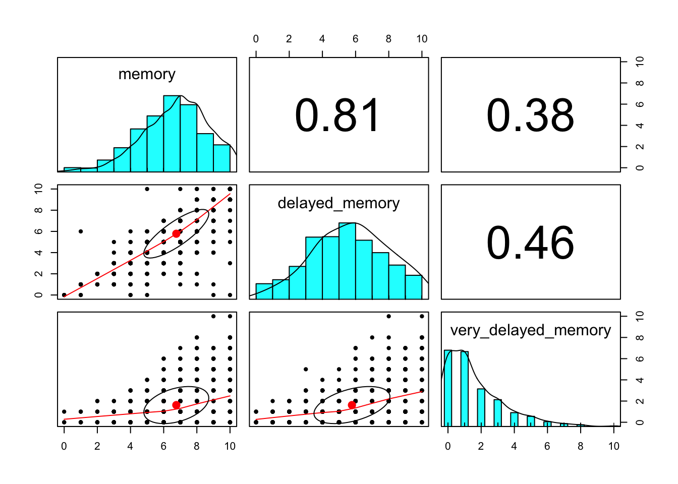
Figure 7: Distributions of memory scores across booth time points.
0.7.3 Change labels of device variable
Longer labels were provided to participants for clarity. However, we will use shorter labels in our analyses and figures.
data = data %>%
  mutate(devicetype = factor(
    devicetype,
    levels = c("Desktop or laptop computer", "Mobile",
               "Tablet (for example, iPad, Galaxy Tablet, Amazon Fire, etc.)"),
    labels = c("Computer", "Mobile", "Tablet")
  ))
0.7.4 Reorder demographic categories
We set the order of ordinal demographic variables, which helps generate more interpretable figures and tables.
data = data %>%
  mutate(edu = factor(edu,
                      levels = c(
                        "Less than 12 years",
                        "High school graduate/GED",
                        "Currently in college/university",
                        "Some college/university, but did not graduate",
                        "Associate degree (2 year)",
                        "College/university degree (4 year)",
                        "Currently in graduate or professional school",
                        "Graduate or professional school degree"))) %>%
  mutate(hhinc = str_remove(hhinc, " a year"),
         hhinc = str_replace_all(hhinc, ",000", "K"),
         hhinc = str_replace_all(hhinc, " to ", "-"),
         hhinc = str_replace_all(hhinc, "less than", "<"),
         hhinc = str_replace_all(hhinc, "more than", ">"))%>%
  mutate(hhinc = factor(hhinc,
                        levels = c(
                          "< $20,000",
                          "$20K-$40K",
                          "$40K-$60K",
                          "$60K-$80K",
                          "$80K-$100K",
                          "$100K-$120K",
                          "$120K-$150K",
                          "$150K-$200K",
                          "$200K-$250K",
                          "$250K-$350K",
                          "$350K-$500K",
                          ">$500K"
                        )))
0.7.5 Long-form dataset
We need one dataset that contains the responses to and timing of the personality items in long form. This will be used for nearly all the statistical models, which will nest items within person. To create this, we first select the responses to the items of different formats. For this set of analyses, we use data collected in both Block 1 and Block 2 – that is, each participant saw the same format for every item during Block 1, but a random format for each item in Block 2.
These variable names have one of four formats: [trait]_[abcd] (for example, talkative_a), [trait]_[abcd]_2 (for example, talkative_a_2), [trait]_[abcd]_3 (e.g., talkative_a_3), or [trait]_[abcd]_3i (e.g., talkative_a_3i). We search for these items using regular expressions.
item_responses = str_subset(
  names(data),
  "^([[:alpha:]])+_[abcd](_2)?(_3)?(i)?$"
)
Similarly, we’ll need to know how long it took participants to respond to these items. These variable names have one of four formats listed above followed by the string page_submit. We search for these items using regular expressions.
item_timing = str_subset(
  names(data),
  "t_([[:alpha:]])+_[abcd](_2)?(_3)?(i)?_page_submit$")
We extract just the participant IDs, delayed memory, and these variables.
items_df = data %>%
  select(proid, condition, time2,
         memory, delayed_memory, very_delayed_memory,
         devicetype,
         all_of(item_responses), all_of(item_timing))
Next we reshape these data into long form. This requires several steps. We’ll need to identify whether each value is a response or timing; we can use the presence of the string t_ for this. Next, we’ll identify the block based on whether the string contains _2 or _3. We also identify whether it ends with i, indicating the item in block 3 started with “I”. Then, we identify the condition based on which letter (a, b, c, or d) follows an underscore. Throughout, we’ll strip the item string of extraneous information until we’re left with only the adjective assessed. Finally, we’ll use spread to create separate columns for the response and the timing variables.
items_df = items_df %>%
  gather(item, value, all_of(item_responses), all_of(item_timing)) %>%
  filter(!is.na(value)) %>%
  # identify whether timing or response
  mutate(variable = ifelse(str_detect(item, "^t_"), "timing", "response"),
         item = str_remove(item, "^t_"),
         item = str_remove(item, "_page_submit$")) %>%
  #identify block
  mutate(
    block = case_when(
      str_detect(item, "_2") ~ "2",
      str_detect(item, "_3") ~ "3",
      TRUE ~ "1"),
    item = str_remove(item, "_[23]")) %>%
  # identify presence of "I"
  mutate(i = case_when(
    str_detect(item, "i$") ~ "Present",
    TRUE ~ "Absent"),
    item = str_remove(item, "i$")) %>%
  separate(item, into = c("item", "format")) %>%
  spread(variable, value)
0.7.5.1 Remove ‘human’ and ‘asleep’
We also remove responses to the adjectives “human” and “asleep”, as these are not personality items per-se and included for the purpose of attention checks.
items_df = items_df %>%
  filter(item != "human") %>%
  filter(item != "asleep")
0.7.5.2 Label formatting conditions
We give labels to the formats, to clarify interpretations and aid table and figure construction.
items_df$format = as.factor(items_df$format)
items_df$format = relevel(items_df$format, ref = "a")
items_df$format = factor(items_df$format,
                               levels = c("a","b","c","d"),
                               labels = c("Adjective\nOnly", "Am\nAdjective", "Tend to be\nAdjective", "Am someone\nwho tends to be\nAdjective"))
0.7.5.3 Identify Big Five mini markers
Big Five Mini Markers (BF-MM) are used only for the yea-saying analyses. We identify these adjectives here so that we can appropriately filter them in or out at each stage of analysis.
bfmm = c("quiet", "unsympathetic", "relaxed", "uncreative",
         "shy", "cold", "unintellectual")
0.7.5.4 Transform seconds
The variable seconds appears to have a very severe right skew (see Figure 8). We log-transform this variable for later analyses.
items_df = items_df %>%
  mutate(seconds_log = log(timing))

range(items_df$timing, na.rm=T)
## [1] 0.000 751.823range(items_df$seconds_log, na.rm=T)## [1] -Inf 6.622501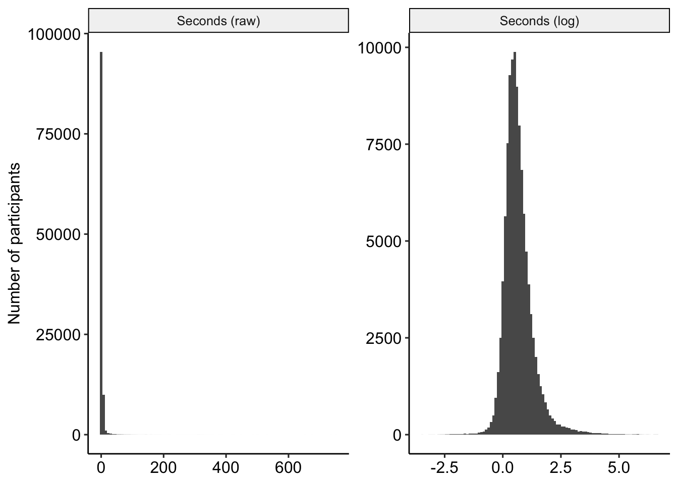
Figure 8: Distribution of seconds, raw and transformed.
0.8 Enjoyment
Finally, in the first wave of data collection, we poll participants about their enjoyment of the study and experience of taking the survey. We extract those columns, along with the condition assigned in Block 1, for later analyses.
enjoy_df = data_t1 %>%
  select(proid, condition, devicetype, enjoy_responding, well_designed_study) %>%
  # convert responses to numeric
  mutate(
    format = tolower(condition),
    format = factor(format,
                    levels = c("a","b","c","d"),
                    labels = c("Adjective\nOnly",
                               "Am\nAdjective",
                               "Tend to be\nAdjective",
                               "Am someone\nwho tends to be\nAdjective")),
    across(
      c(enjoy_responding, well_designed_study),
      ~case_when(
        . == "Very inaccurate"       ~ 1,
        . == "Moderately inaccurate" ~ 2,
        . == "Slightly inaccurate"   ~ 3,
        . == "Slightly accurate"     ~ 4,
        . == "Moderately accurate"   ~ 5,
        . == "Very accurate"         ~ 6,
        TRUE ~ NA_real_
      )
    )
  ) %>%
  filter(proid %in% items_df$proid)
0.9 Save files
# check if folder exists. if not create it
if (!file.exists(here("objects/"))){
    dir.create(here("objects/"))
}
save(reverse, file = here("objects/reverse_vector.Rds"))
save(bfmm, file = here("objects/bfmm.Rds"))
save(data, file = here("objects/cleaned_data.Rds"))
save(items_df, file = here("objects/items_df.Rds"))
save(enjoy_df, file = here("objects/enjoy_df.Rds"))