Test-retest reliability

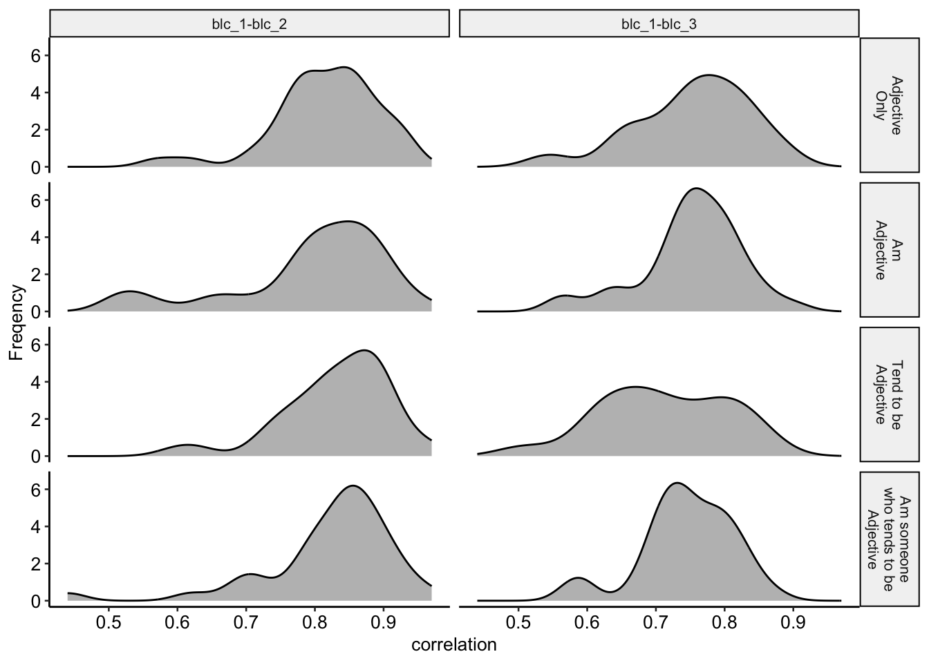
We also evaluated test-retest reliability within formats (within session and over two weeks); we expecte slightly higher test-retest reliability for item wording formats that are more specific – formats #3 and #4 above vs the use of adjectives alone. However, we found that test-retest reliability did not differ as a function of item format.

We also considered the effect of performance on the word recall task on retest reliability.

The data structure needed for these analyses is in wide-format. That is, we require one column for each time point. In addition, we hope to examine reliability within format, which requires selecting only the response options which match the original, Block 1, assessment.

items_df = items_df %>% 
  mutate(condition = tolower(condition)) %>% 
  mutate(condition = factor(condition, 
                            levels = c("a", "b", "c", "d"),
                            labels = c("Adjective\nOnly", "Am\nAdjective", 
                                       "Tend to be\nAdjective", 
                                       "Am someone\nwho tends to be\nAdjective")))

items_matchb1 = items_df %>% 
  mutate(across(c(format, condition), as.character)) %>% 
  filter(format == condition) %>% 
  mutate(block = paste0("block_", block)) %>% 
  select(-timing, -seconds_log, -i) %>% 
  spread(block, response)

We standardize responses within each block – this allows us to use a regression framework yet interpret the slopes as correlations.

items_matchb1 = items_matchb1 %>% 
  mutate(across(
    starts_with("block"), ~(.-mean(., na.rm=T))/sd(., na.rm = T)
  ))

We also standardize the memory scores for ease of interpretation.

items_matchb1 = items_matchb1 %>% 
  mutate(across(
    ends_with("memory"), ~(.-mean(., na.rm=T))/sd(., na.rm = T)
  ))

Test-retest reliability (all items pooled)

To estimate the reliability coefficients, we use a multilevel model, predicting the latter block from the earlier one. These models nest responses within participant, allowing us to estimate standard errors which account for the dependency of scores. Results are shown in Table @ref(tab:testretest7b).

tr_mod1_b1b2 = glmmTMB(block_2 ~ block_1 + (1 |proid), data = items_matchb1)
tr_mod1_b1b3 = glmmTMB(block_3 ~ block_1 + (1 |proid), data = items_matchb1)

Test-retest estimates from multilevel models

Assessments	Slope coefficient
Block 1 - Block 2	0.85 [0.84, 0.86]
Block 1 - Block 3	0.78 [0.77, 0.79]

Test-retest reliability (all items pooled, moderated by memory)

Here we fit models moderated by memory – that is, perhaps the test-retest coefficient is affected by the memory of the participant. Results are shown in Table @ref(tab:testretest8b)

tr_mod2_b1b2 = glmmTMB(block_2 ~ block_1*delayed_memory +
                      (1 |proid),
                    data = items_matchb1)
tr_mod2_b1b3 = glmmTMB(block_3 ~ block_1*very_delayed_memory +
                      (1 |proid),
                    data = items_matchb1)

Effect of memory on test-retest

Term	Interpretation	Block 1 - Block 2	Block 1 - Block 3
block_1	Test-retest at average memory	0.85 [0.84, 0.86]	0.78 [0.77, 0.79]
block_1:memory	Change in test-retest by increase in memory	0.03 [0.02, 0.04]	0.01 [0.00, 0.02]
memory	Effect of memory on response	0.01 [0.00, 0.03]	0.01 [-0.01, 0.02]

We also extract the simple slopes estimates of these models, which allow us to more explicitly identify and compare the test-retest correlations.

Block 1/Block 2

mem_list = list(delayed_memory = c(-1,0,1))

emtrends(tr_mod2_b1b2,
         pairwise~delayed_memory,
         var = "block_1",
         at = mem_list)

$emtrends
 delayed_memory block_1.trend      SE  df asymp.LCL asymp.UCL
             -1         0.821 0.00745 Inf     0.807     0.836
              0         0.854 0.00534 Inf     0.843     0.864
              1         0.886 0.00749 Inf     0.872     0.901

Confidence level used: 0.95 

$contrasts
 contrast                             estimate      SE  df z.ratio p.value
 (delayed_memory-1) - delayed_memory0  -0.0324 0.00522 Inf  -6.206  <.0001
 (delayed_memory-1) - delayed_memory1  -0.0648 0.01040 Inf  -6.206  <.0001
 delayed_memory0 - delayed_memory1     -0.0324 0.00522 Inf  -6.206  <.0001

P value adjustment: tukey method for comparing a family of 3 estimates 

Block 1/Block 3

mem_list = list(very_delayed_memory = c(-1,0,1))

emtrends(tr_mod2_b1b3,
         pairwise~very_delayed_memory,
         var = "block_1",
         at = mem_list)

$emtrends
 very_delayed_memory block_1.trend      SE  df asymp.LCL asymp.UCL
                  -1         0.770 0.00477 Inf     0.760     0.779
                   0         0.781 0.00340 Inf     0.775     0.788
                   1         0.793 0.00474 Inf     0.784     0.802

Confidence level used: 0.95 

$contrasts
 contrast                                       estimate      SE  df z.ratio
 (very_delayed_memory-1) - very_delayed_memory0  -0.0115 0.00332 Inf  -3.463
 (very_delayed_memory-1) - very_delayed_memory1  -0.0230 0.00665 Inf  -3.463
 very_delayed_memory0 - very_delayed_memory1     -0.0115 0.00332 Inf  -3.463
 p.value
  0.0015
  0.0015
  0.0015

P value adjustment: tukey method for comparing a family of 3 estimates 

Test-retest reliability (all items pooled, by format)

We fit these same models, except now we moderate by format, to determine whether the test-retest reliability differs as a function of item wording.

tr_mod3_b1b2 = glmmTMB(block_2 ~ block_1*condition + (1 |proid),
                    data = items_matchb1)
tr_mod3_b1b3 = glmmTMB(block_3 ~ block_1*condition + (1 |proid),
                    data = items_matchb1)

aov(tr_mod3_b1b2)

Call:
   aov(formula = tr_mod3_b1b2)

Terms:
                 block_1 condition    proid block_1:condition Residuals
Sum of Squares  6896.958     0.836  324.094             0.422  2008.689
Deg. of Freedom        1         3      971                 3      8253

Residual standard error: 0.4933447
3 out of 982 effects not estimable
Estimated effects may be unbalanced
27818 observations deleted due to missingness

aov(tr_mod3_b1b3)

Call:
   aov(formula = tr_mod3_b1b3)

Terms:
                  block_1 condition     proid block_1:condition Residuals
Sum of Squares  21651.611     7.361  1062.946             1.640 10829.442
Deg. of Freedom         1         3       879                 3     32667

Residual standard error: 0.5757692
3 out of 890 effects not estimable
Estimated effects may be unbalanced
3496 observations deleted due to missingness

We also extract the simple slopes estimates of these models, which allow us to more explicitly identify and compare the test-retest correlations.

Block 1/Block 2

emtrends(tr_mod3_b1b2, pairwise ~ condition, var = "block_1")

$emtrends
  condition                             block_1.trend     SE  df asymp.LCL
 Adjective\nOnly                                0.852 0.0107 Inf     0.831
 Am\nAdjective                                  0.848 0.0108 Inf     0.827
 Am someone\nwho tends to be\nAdjective         0.865 0.0104 Inf     0.844
 Tend to be\nAdjective                          0.848 0.0105 Inf     0.828
 asymp.UCL
     0.873
     0.869
     0.885
     0.869

Confidence level used: 0.95 

$contrasts
   contrast                                                      estimate
 Adjective\nOnly - Am\nAdjective                                 0.004793
 Adjective\nOnly - Am someone\nwho tends to be\nAdjective       -0.012283
 Adjective\nOnly - Tend to be\nAdjective                         0.004220
 Am\nAdjective - Am someone\nwho tends to be\nAdjective         -0.017076
 Am\nAdjective - Tend to be\nAdjective                          -0.000573
 Am someone\nwho tends to be\nAdjective - Tend to be\nAdjective  0.016503
     SE  df z.ratio p.value
 0.0152 Inf   0.316  0.9891
 0.0149 Inf  -0.827  0.8419
 0.0150 Inf   0.282  0.9922
 0.0149 Inf  -1.143  0.6628
 0.0151 Inf  -0.038  1.0000
 0.0147 Inf   1.120  0.6772

P value adjustment: tukey method for comparing a family of 4 estimates 

Block 1/Block 3

emtrends(tr_mod3_b1b3, pairwise ~ condition, var = "block_1")

$emtrends
  condition                             block_1.trend      SE  df asymp.LCL
 Adjective\nOnly                                0.785 0.00676 Inf     0.772
 Am\nAdjective                                  0.791 0.00678 Inf     0.777
 Am someone\nwho tends to be\nAdjective         0.778 0.00661 Inf     0.765
 Tend to be\nAdjective                          0.772 0.00682 Inf     0.758
 asymp.UCL
     0.798
     0.804
     0.791
     0.785

Confidence level used: 0.95 

$contrasts
   contrast                                                     estimate
 Adjective\nOnly - Am\nAdjective                                -0.00581
 Adjective\nOnly - Am someone\nwho tends to be\nAdjective        0.00729
 Adjective\nOnly - Tend to be\nAdjective                         0.01309
 Am\nAdjective - Am someone\nwho tends to be\nAdjective          0.01310
 Am\nAdjective - Tend to be\nAdjective                           0.01890
 Am someone\nwho tends to be\nAdjective - Tend to be\nAdjective  0.00580
      SE  df z.ratio p.value
 0.00956 Inf  -0.608  0.9296
 0.00944 Inf   0.773  0.8668
 0.00958 Inf   1.366  0.5206
 0.00945 Inf   1.386  0.5080
 0.00959 Inf   1.970  0.1995
 0.00948 Inf   0.612  0.9284

P value adjustment: tukey method for comparing a family of 4 estimates 

Test-retest reliability (items separated, by format)

To assess test-retest reliability for each item, we can rely on more simple correlation analyses, as each participant only contributed one response to each item in each block. We first not the sample size coverage for these comparisons:

items_matchb1 %>%
  group_by(item, condition) %>%
  count() %>%
  ungroup() %>%
  full_join(expand_grid(item = unique(items_matchb1$item),
                        condition = unique(items_matchb1$condition))) %>%
  mutate(n = ifelse(is.na(n), 0, n)) %>%
  summarise(
    min = min(n),
     max = max(n),
    mean = mean(n),
    median = median(n)
  )

# A tibble: 1 × 4
    min   max  mean median
  <int> <int> <dbl>  <dbl>
1   239   248  244.    244

items_cors = items_matchb1 %>%
  select(item, condition, contains("block")) %>%
  group_by(item, condition) %>%
  nest() %>%
   mutate(cors = map(data, psych::corr.test, use = "pairwise"),
         cors = map(cors, print, short = F),
         cors = map(cors, ~.x %>% mutate(comp = rownames(.)))) %>%
  select(item, condition, cors) %>%
  unnest(cols = c(cors))

The test-retest correlations of each item-format combination are presented in Table @ref(tab:testretest17). We also visualize these correlations in Figure @ref(fig:testretest18),

Test-retest correlations for each item and condition.

		Adjective Only		Am Adjective		Tend to be		Am someone who tends to be
Item	Reverse scored?	5 min	2 weeks	5 min	2 weeks	5 min	2 weeks	5 min	2 weeks
active	N	0.79	0.73	0.87	0.77	0.89	0.71	0.86	0.78
adventurous	N	0.91	0.79	0.82	0.76	0.89	0.67	0.88	0.79
broadminded	N	0.83	0.68	0.78	0.63	0.80	0.67	0.77	0.67
calm	N	0.85	0.74	0.80	0.74	0.76	0.62	0.81	0.74
caring	N	0.78	0.76	0.65	0.72	0.77	0.64	0.85	0.72
cautious	N	0.57	0.54	0.53	0.56	0.73	0.51	0.72	0.58
cold	N	0.93	0.76	0.72	0.72	0.95	0.68	0.90	0.70
creative	N	0.75	0.82	0.84	0.80	0.90	0.86	0.85	0.87
curious	N	0.76	0.66	0.69	0.57	0.87	0.62	0.44	0.59
friendly	N	0.71	0.81	0.87	0.71	0.73	0.79	0.84	0.79
hardworking	N	0.83	0.78	0.89	0.76	0.88	0.79	0.86	0.81
helpful	N	0.77	0.65	0.89	0.80	0.74	0.70	0.88	0.74
imaginative	N	0.80	0.80	0.87	0.79	0.82	0.84	0.91	0.83
intelligent	N	0.84	0.83	0.84	0.71	0.86	0.64	0.84	0.71
lively	N	0.86	0.75	0.83	0.81	0.83	0.74	0.79	0.75
organized	N	0.85	0.87	0.93	0.86	0.83	0.82	0.89	0.83
outgoing	N	0.90	0.89	0.91	0.90	0.84	0.85	0.84	0.84
quiet	N	0.93	0.83	0.81	0.80	0.88	0.69	0.68	0.73
relaxed	N	0.85	0.69	0.78	0.75	0.60	0.61	0.83	0.70
responsible	N	0.77	0.78	0.79	0.76	0.82	0.68	0.71	0.75
selfdisciplined	N	0.76	0.81	0.76	0.75	0.89	0.75	0.77	0.80
shy	N	0.85	0.85	0.96	0.85	0.91	0.80	0.94	0.78
softhearted	N	0.78	0.79	0.85	0.77	0.88	0.77	0.87	0.78
sophisticated	N	0.88	0.75	0.80	0.76	0.88	0.68	0.80	0.75
sympathetic	N	0.80	0.75	0.65	0.74	0.79	0.79	0.85	0.72
talkative	N	0.90	0.81	0.86	0.76	0.83	0.80	0.87	0.75
thorough	N	0.79	0.64	0.78	0.65	0.81	0.61	0.81	0.70
thrifty	N	0.86	0.74	0.81	0.79	0.90	0.62	0.80	0.69
uncreative	N	0.82	0.71	0.53	0.74	0.77	0.74	0.70	0.81
unintellectual	N	0.87	0.71	0.57	0.63	0.63	0.51	0.62	0.59
unsympathetic	N	0.72	0.55	0.51	0.73	0.84	0.63	0.80	0.73
warm	N	0.81	0.77	0.90	0.79	0.87	0.73	0.92	0.75
careless	Y	0.62	0.65	0.77	0.68	0.86	0.61	0.85	0.72
impulsive	Y	0.78	0.66	0.82	0.74	0.78	0.68	0.92	0.71
moody	Y	0.93	0.88	0.89	0.83	0.97	0.81	0.89	0.82
nervous	Y	0.88	0.83	0.85	0.80	0.91	0.83	0.97	0.78
reckless	Y	0.85	0.76	0.86	0.81	0.82	0.71	0.83	0.72
worrying	Y	0.81	0.84	0.89	0.83	0.89	0.83	0.88	0.80

Test-retest correlations of specific items across word format.