Does the internal consistency of Big Five traits vary by item wording?
Last updated 2023-08-11
We calculate and report Cronbach’s alpha for all formats using data from Blocks 1 and 2. This will include both the average split-half reliability, as well as the 95% confidence interval. Differences in internal consistency will be considered statistically significant if the confidence intervals of two formats do not overlap. We will also show the distribution of all possible split halves for each of the four formats.
We start by creating a wide-format of the dataset using only the Block 1 data.
items_wide = items_df %>%
  # only blocks 1 and 2
  filter(block %in% c(1,2)) %>%
  #only need these variables
  select(proid, block, condition, item, response) %>%
  # to wide form
  spread(item, response)
Next, we identify the items associated with each trait. These come from the Health and Retirement Study Psychosocial and Lifestyle Questionnaire 2006-2016 user guide, which can be found at this link.
Extra = c("outgoing", "friendly", "lively", "active" ,"talkative")
Agree = c("helpful", "warm", "caring", "softhearted", "sympathetic")
Consc = c("reckless", "organized", "responsible", "hardworking", "selfdisciplined",
          "careless", "impulsive", "cautious", "thorough", "thrifty")
Neuro = c("moody", "worrying", "nervous", "calm")
Openn = c("creative", "imaginative", "intelligent", "curious", "broadminded",
          "sophisticated", "adventurous")
0.1 Calculate Cronbach’s alpha for each format
We start by grouping data by condition and then nesting, to create separate data frames for each of the four formats.
format_data = items_wide %>%
  group_by(condition) %>%
  nest() %>%
  ungroup()
Next we create separate datasets for each of the five personality traits.
format_data = format_data %>%
  mutate(
    data_Extra = map(data, ~select(.x, all_of(Extra))),
    data_Agree = map(data, ~select(.x, all_of(Agree))),
    data_Consc = map(data, ~select(.x, all_of(Consc))),
    data_Neuro = map(data, ~select(.x, all_of(Neuro))),
    data_Openn = map(data, ~select(.x, all_of(Openn)))
    )
We gather these datasets into a single column, for ease of use.
format_data = format_data %>%
  select(-data) %>%
  gather(variable, data, starts_with("data")) %>%
  mutate(variable = str_remove(variable, "data_"))
Next we apply the alpha and omega functions to the datasets. We do not need to use the check.keys function, as items were reverse-scored during the cleaning process.
format_data = format_data %>%
  mutate(
    nvar = map_dbl(data, ncol),
    alpha = map(data, psych::alpha),
    omega = map(data, psych::omega, plot = F))
0.2 Alpha
We extract the estimated confidence intervals. The final summary of results is presented in Table 1 and Figure 1.
format_alpha = format_data %>%
  mutate(alpha_list = map(alpha, "total"),
         alpha_est = map_dbl(alpha_list, "raw_alpha"),
         se_est = map_dbl(alpha_list, "ase"),
         lower_est = alpha_est - (1.96*se_est),
upper_est = alpha_est + (1.96*se_est)) | label | A | B | C | D |
|---|---|---|---|---|
| Extraversion (5 descriptors) | 0.80 [0.77, 0.82] | 0.82 [0.80, 0.85] | 0.84 [0.82, 0.86] | 0.81 [0.78, 0.83] |
| Agreeableness (5 descriptors) | 0.90 [0.89, 0.91] | 0.90 [0.88, 0.91] | 0.90 [0.88, 0.91] | 0.92 [0.91, 0.93] |
| Conscientiousness (10 descriptors) | 0.83 [0.80, 0.85] | 0.85 [0.82, 0.87] | 0.80 [0.78, 0.83] | 0.84 [0.81, 0.86] |
| Neuroticism (4 descriptors) | 0.83 [0.81, 0.86] | 0.86 [0.84, 0.88] | 0.82 [0.79, 0.84] | 0.83 [0.81, 0.86] |
| Openness (7 descriptors) | 0.76 [0.72, 0.79] | 0.68 [0.64, 0.73] | 0.77 [0.73, 0.80] | 0.72 [0.68, 0.76] |
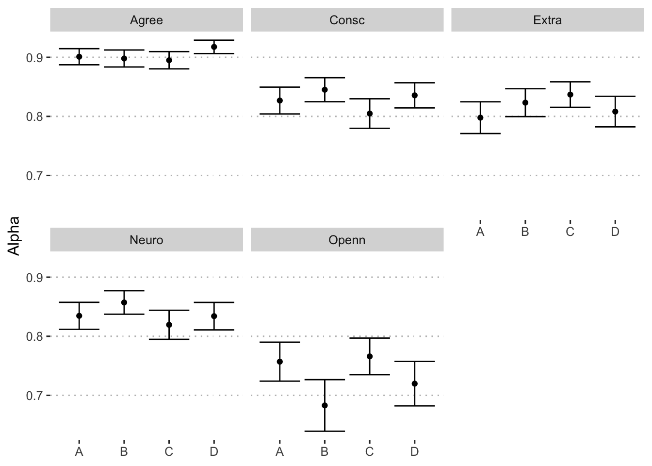
Figure 1: Estimates of Cronbach’s alpha across format and trait.
0.3 Split-half reliability
Alpha is the average split-half reliability; given space, it can be useful to report the distribution of all split-half reliability estimates. We use the splitHalf function to calculate those. We use smoothed correlation matrices here because when developing code on the pilot data, we had non-positive definite correlation matrices. See Figure 2 for these distributions.
format_split = format_data %>%
  mutate(cor_mat = map(data, cor),
         cor_mat = map(cor_mat, cor.smooth)) %>%
  mutate(splithalf = map(cor_mat, splitHalf, raw = T))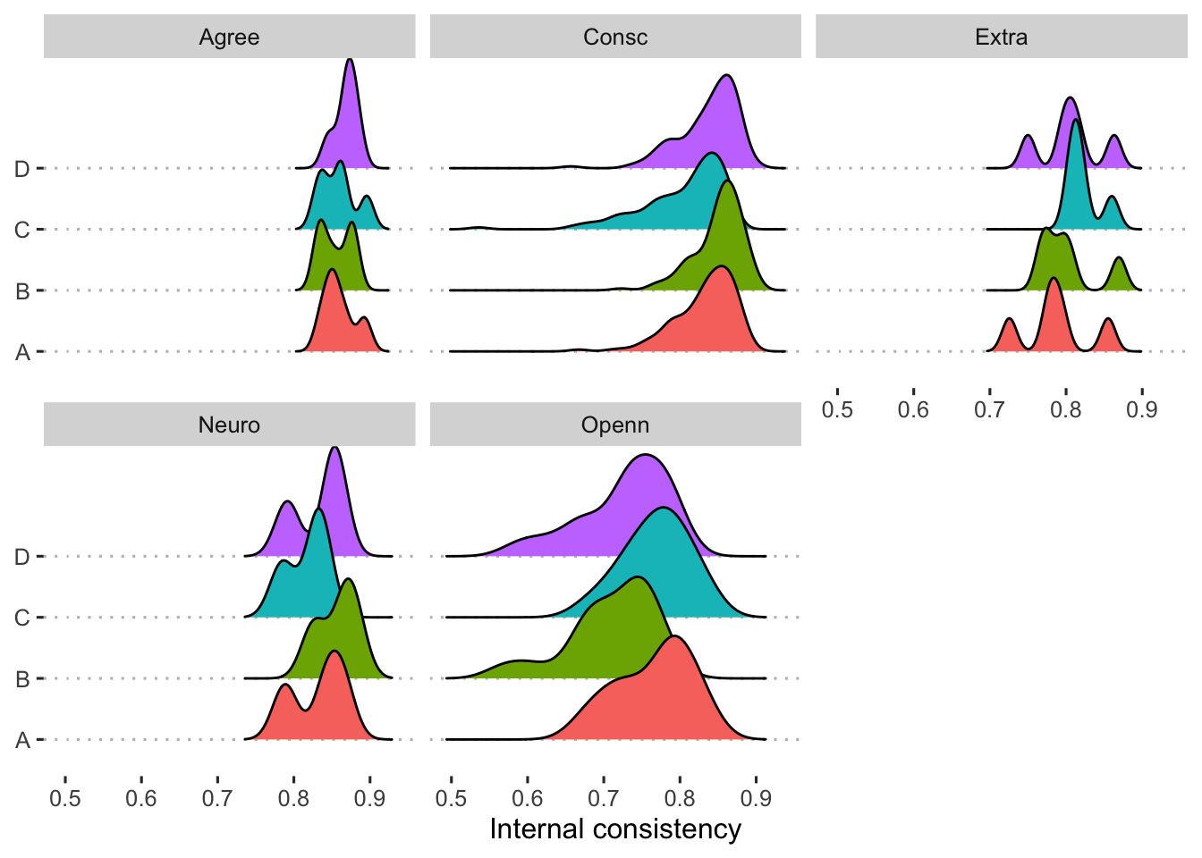
Figure 2: Distribution of split-half reliabilities
0.4 Omega
We extract the estimated confidence intervals.The final summary of results is presented in Table 1 and Figure 1.
format_omega = format_data %>%
mutate(omega_h = map_dbl(omega, "omega_h")) | label | A | B | C | D |
|---|---|---|---|---|
| Extraversion (5 descriptors) | 0.75 | 0.76 | 0.77 | 0.75 |
| Agreeableness (5 descriptors) | 0.89 | 0.82 | 0.82 | 0.88 |
| Conscientiousness (10 descriptors) | 0.67 | 0.65 | 0.54 | 0.55 |
| Neuroticism (4 descriptors) | 0.80 | 0.84 | 0.81 | 0.79 |
| Openness (7 descriptors) | 0.62 | 0.56 | 0.66 | 0.53 |
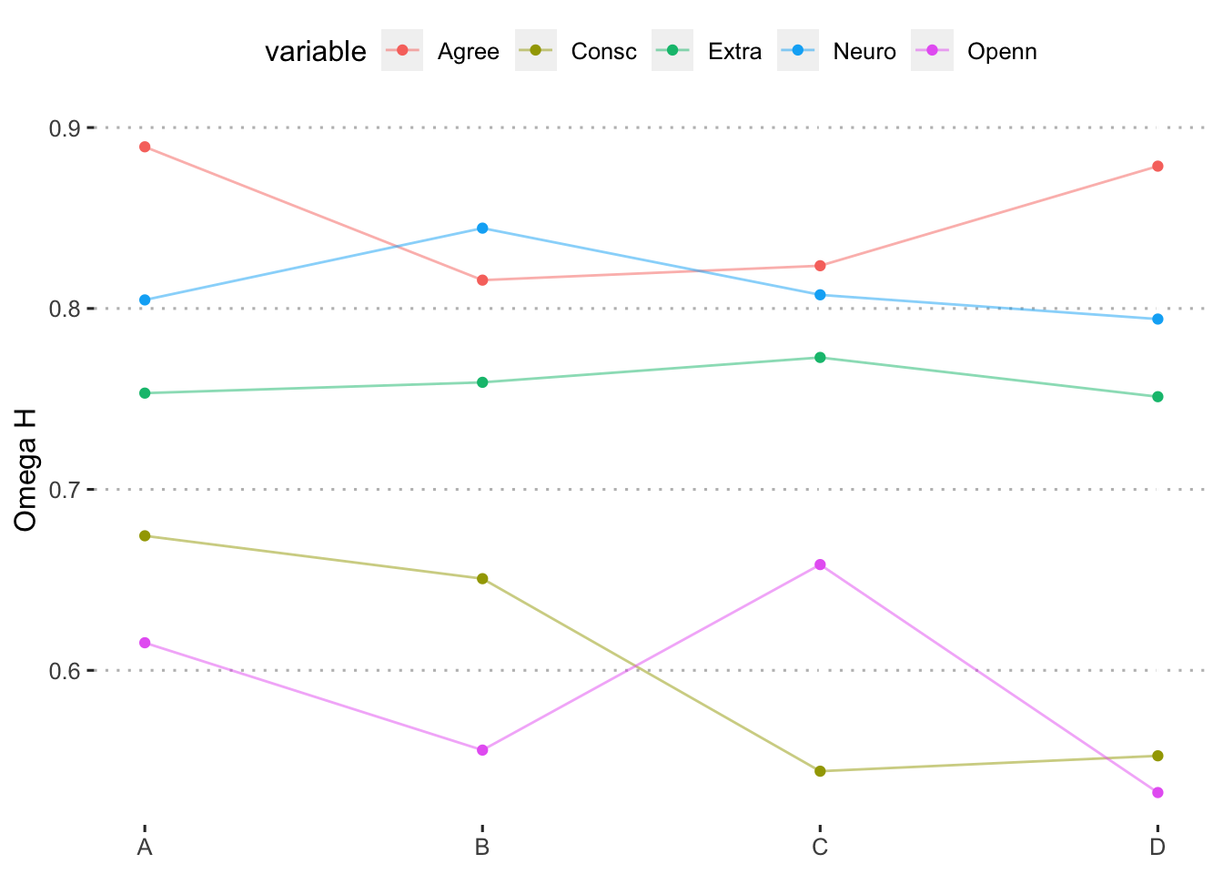
Figure 3: Estimates of omega hierarchical across format and trait.